InfuseLoop

Better depth scaling for parallel looped transformers.

Go Deeper, Stay Fast

Prompt

Looped Transformer (LT)

Efficiency ✕Quality ✓

Parallel Looped Transformer (PLT)

Efficiency ✓Quality ✕

InfuseLoop

Efficiency ✓Quality ✓

Simulated playback at measured speed ratios. Quality marks describe this example.
Measured results
LTPLTInfuseLoop

Better text prediction

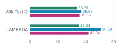
Measured eight-loop perplexity on WikiText-2 and LAMBADA: InfuseLoop improves over PLT on both benchmarks, while LT has the lowest perplexity.
Perplexity ↓ · Lower is better

Higher task accuracy

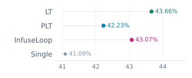
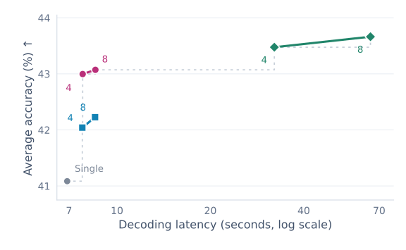
Seven-task average accuracy: Single 41.09 percent, PLT 42.23 percent, InfuseLoop 43.07 percent and LT 43.66 percent.
Seven-task average accuracy (%) ↑

PLT-like decoding latency

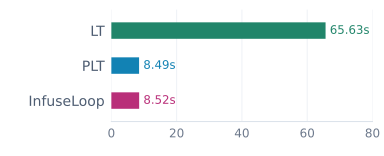
Measured eight-loop decode-only latency: LT 65.63 seconds, PLT 8.49 seconds, InfuseLoop 8.52 seconds. InfuseLoop is close to PLT and much faster than serial LT.
Decoding latency (seconds) ↓
Source data

The charts compare measured eight-loop quality and decode-only latency, using the 0.6B models trained on 6B tokens. Latency uses one GB200 at batch size 32 with 2K-token prompts and outputs, separately from the illustrative playback.

These continuations are unchanged checkpoint outputs selected from 64 prompts. The animation uses uniform token intervals scaled from an earlier, validated 256-token benchmark on one GB200: about 7.7Ă— faster for InfuseLoop than LT, and nearly the same rate as PLT. It is a simulated illustration, not a timing measurement of this passage. One slowdown factor applies to every model.
Why InfuseLoop

  • Depth is useful, but serial loops are costly. LT reuses one backbone for additional computation; PLT overlaps loop stages across predictions to reduce the sequential decoding cost.
  • Parallel execution leaves useful states unrouted. Vanilla PLT passes only the preceding in-trajectory state between loops, leaving completed neighboring-trajectory outputs outside the recurrent input.
  • Additional loops need better information flow. Our vanilla PLT runs exhibit training spikes and limited depth scaling, motivating richer inputs from representations the pipeline has already computed.
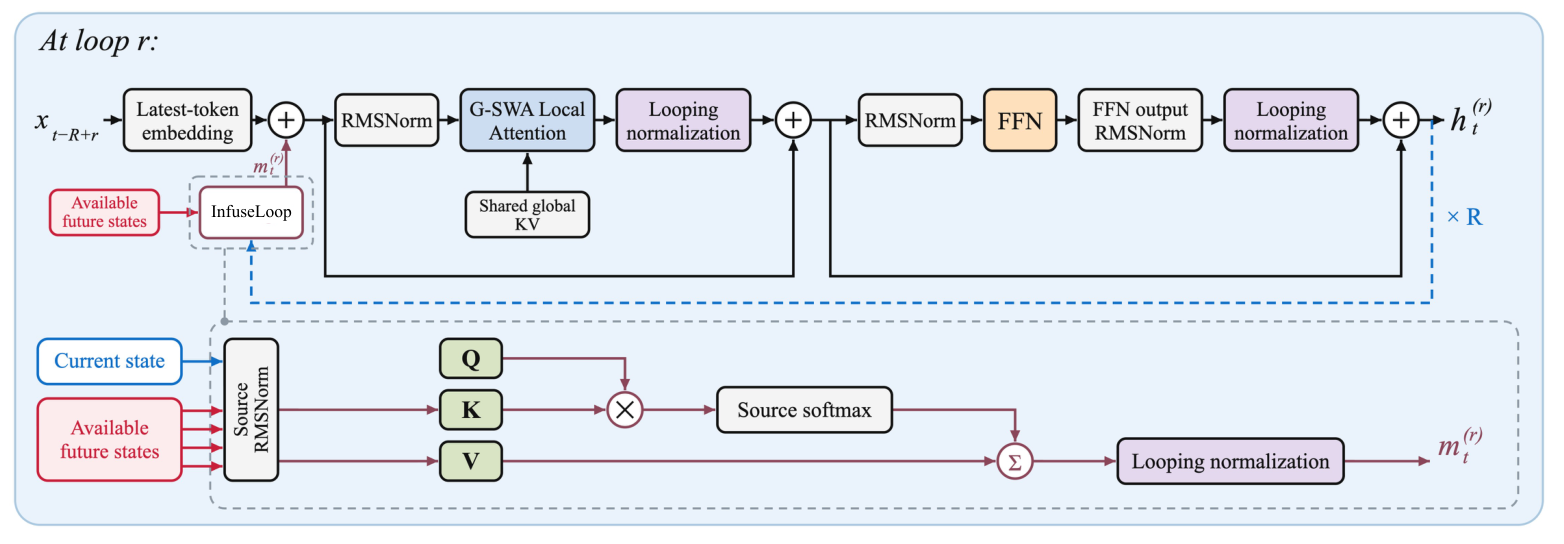
InfuseLoop overview: completed cross-trajectory states are aggregated into recurrent inputs, with attention, FFN and shared global KV.
InfuseLoop overview. Enrich recurrent inputs with completed cross-trajectory states while preserving the parallel backbone schedule.

How it works

  • Use non-stale states. Aggregate outputs from the immediately preceding execution cycle to reuse the freshest available contextual representations.
  • Route through shallower future states. Select states from later prediction trajectories at shallower loops, preserving token-parallel training and identical training–inference routing without approximations.

Information flow

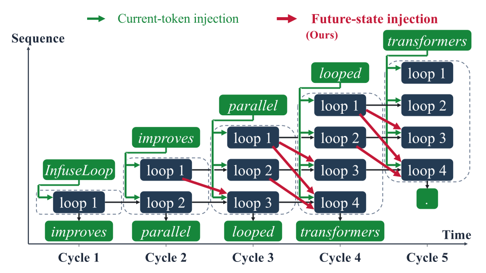
InfuseLoop information flow across execution cycles: green arrows inject the current token and red arrows route completed states across prediction trajectories.
Reuse completed computations. Green arrows inject the current token; red arrows connect available states across prediction trajectories.

State availability

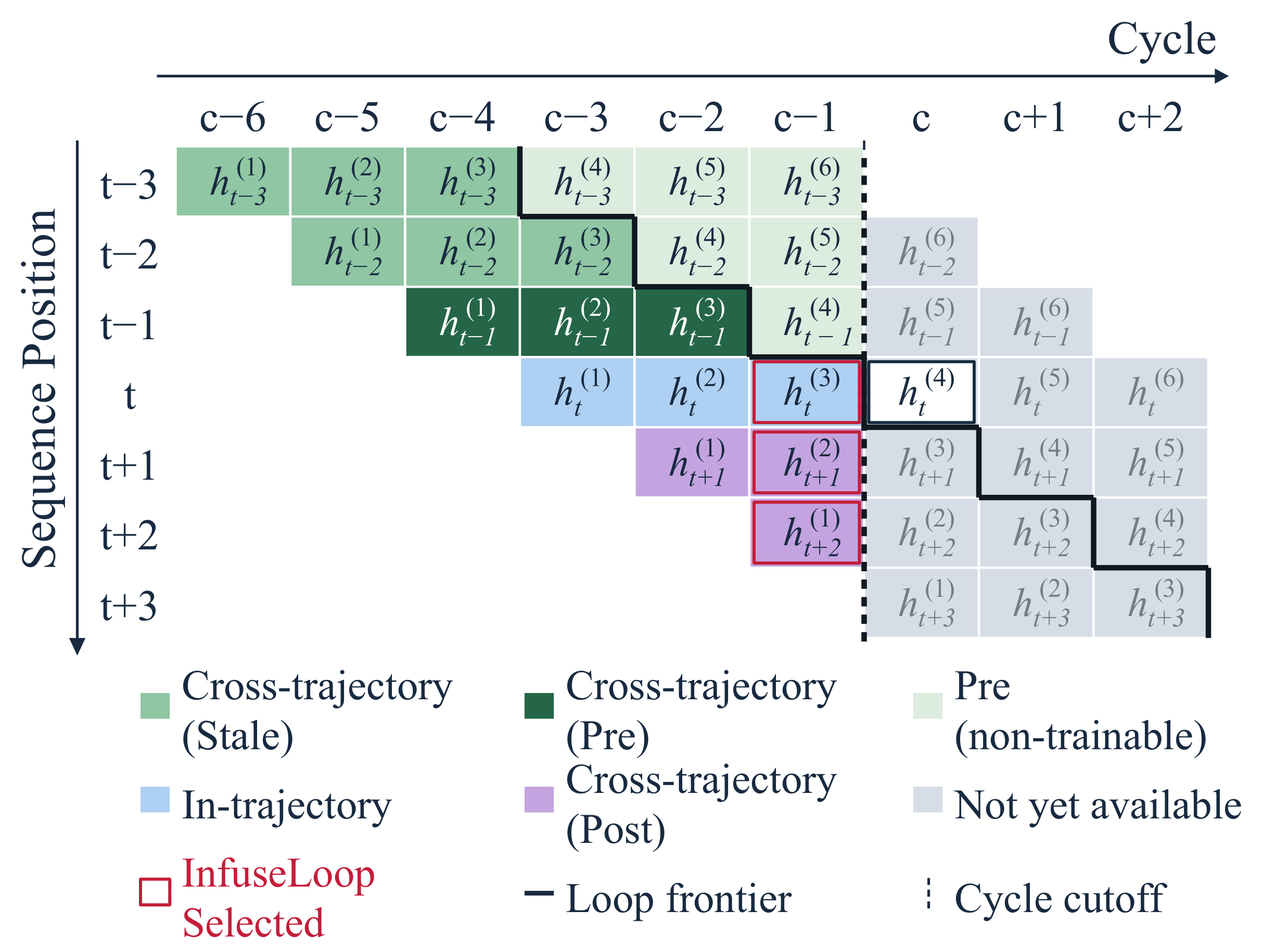
State-availability diagram for a fourth-loop update: red outlines select the previous-cycle base state and shallower future states, while gray cells have not yet been computed.
Select the previous-cycle snapshot. Red outlines mark the selected base and shallower future states; gray cells are not yet available.

Depth scalability and Pareto efficiency

InfuseLoop improves depth scalability while preserving efficient parallel execution, expanding the performance–latency Pareto frontier of looped Transformers.
LTPLTInfuseLoopSingle

Depth scaling

Language modeling improves with depth

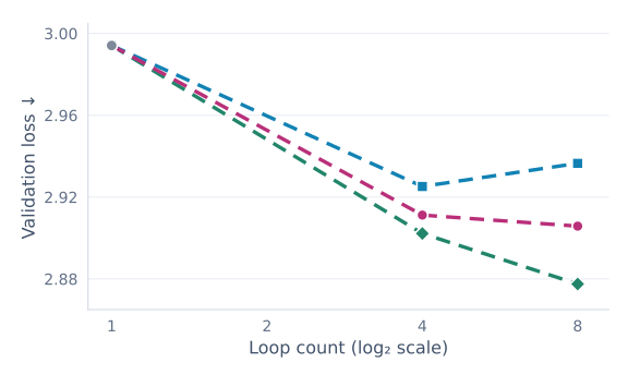
Loop count versus validation loss for LT, PLT and InfuseLoop, at measured depths one, four and eight.
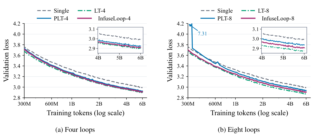
Loop count versus validation loss; lower is better. InfuseLoop continues to reduce loss as depth increases, while vanilla PLT regresses between four and eight loops.

Downstream gains persist across depths

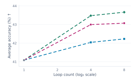
Loop count versus seven-task average accuracy. InfuseLoop stays above PLT at four and eight loops, while LT has the highest accuracy.
Loop count versus average accuracy across seven tasks; higher is better. InfuseLoop retains its advantage over vanilla PLT at both evaluated recurrent depths.

Performance–latency Pareto frontiers

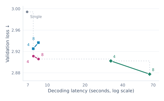
Performance–latency frontier: validation loss

Decode latency versus validation loss, showing the measured frontier and four- and eight-loop configurations.
Decoding latency versus loss; lower left is better. InfuseLoop adds lower-loss configurations near PLT's latency. Its four-loop model dominates eight-loop PLT.

Performance–latency frontier: downstream accuracy

Decode latency versus seven-task accuracy. InfuseLoop improves the low-latency frontier, while LT provides higher quality at substantially higher latency.
Decoding latency versus average accuracy; upper left is better. InfuseLoop improves the low-latency frontier. LT achieves higher absolute quality at substantially greater latency.

Long-context efficiency

Throughput approaches the non-looped baseline

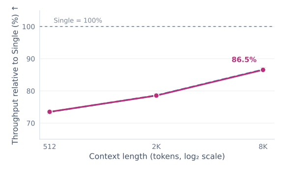
At batch size 32, eight-loop InfuseLoop closely tracks PLT and retains 86.5 percent of Single throughput at an 8192-token context.
Context length versus throughput relative to Single; higher is better. At eight loops and batch size 32, InfuseLoop closely tracks PLT and retains 86.5% of Single's throughput at 8K context.

Shared KV keeps additional cache storage bounded

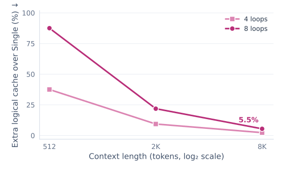
Analytical logical-cache overhead over Single at four and eight loops with window 64, declining with context length to 2.3 and 5.5 percent at 8K context.
Context length versus extra logical cache storage over Single; lower is better. With a 64-token local window, eight-loop overhead falls to 5.5% at 8K context. This is analytical cache storage, excluding model weights and workspaces.
Training curves, measurement details, and source dataValidation-loss trajectories for four-loop and eight-loop models

Each quality point is a separately trained 0.6B model using 6B tokens. The latency benchmark uses one GB200 at batch size 32, 2K-token prompts and outputs, and the median of three decode-only runs after prefill. Context sensitivity uses 64-cycle windows, separately from the full-generation latency benchmark. CUDA Graphs, FA4, and custom G-SWA kernels are used. Cache overhead is computed from shared global KV, loop-local windows, and aggregation states. Larger and MoE models remain untested.